Chapter 2 Data types and Data structures

2.1 Lets Begin

We assume that R or Rstudio is installed. R is an integrated suite of software facilities for data manipulation, calculation and graphical display.

In all the documents, the R codes written in shaded box are the codes which you can copy and try in R console. The results are shown in unshaded box.

Lets first understand the difference between expression and assignment statements in R.

2.2 Expression

Expressions are evaluated, results are printed. Results are not stored.

Semicolon ‘;’ is optional to end a statement. Its recommended to give ; at the end of each statement.

# (Hash), is used to comment single line.

# Space around + is optional but code looks clean. So recommended. Statement is not executed.
2 + 5;

## [1] 7

Lets explore some more. You can use R console as calculator.

2 * 3;

## [1] 6

2.3 Assignment

An assignment is a statement which is evaluated and result is stored but results of the evaluation are not printed on console.

Right hand side is evaluated whose results is stored in left hand side.

Either use = or <- as Assignment operator.

# In this example value of x will be 2.
x=2; # 2 will be assigned to x; Value of x will not be printed on console.
x <- 2+5;
x;

## [1] 7

2.4 Working directory

# Present working directory
getwd();

## [1] "/home/priyabrata/learn/github/bookdown-demo-master"

# setwd(): change the working directory by passing path of new directory.
# Enclose the path between " " (double quotes)
setwd("/home/user/")

2.5 List of objects in workspace/environment

# Lists all objects/variables created in the workspace/environment
ls();

## [1] "x"

# rm():Delete provided object
rm(x);

2.6 getting help in R

# Access to R documentation
help.start()
# Help on mean
?mean
help(solve)
# More depth search
??mean
# Explore examples on mean
example(mean);

2.6.1 Some things to Remember

R is case sensitive
; is ends a statement
# is used to comment

2.7 Data Types

Every programming language deals with data. It is important to understand what kind of data you are dealing with and how you are going to store this. You can refer these two concepts as Data types and Data structures respectively. First we will start with data types and then move to data structures.

Data can be either in the form of integer, numeric, character or logical/boolean (TRUE/FALSE). Thus based on kind of data, data types in R can be broadly categorized into 5 categories

Integer (int): Represents integer data such as -2, 0, 2.
Numeric (num): Represents integers as well as decimals such as 2, 2.3, -2.3.
Logical (logi): Represents boolean values such as TRUE and FALSE. One can also write T and F respectively. It is important to note about the case sensitivity while dealing with logical/boolean data. If you write true/false/True/False/t/f, it will not considered as logical data types (Everything has to be capital T/TRUE/F/FALSE).
Character (chr): Represents single character (e.g. ‘M’, ‘F’) or multi-character string (e.g. ‘ABC’,‘DEF’) data. Both single (’) and double quotes (“) can be used to store character data (‘ABC’,”ABC").
Factor: Stores categorical data. We will explain this in detail in later sections.

2.8 Data Structures

Depending on the data, it can be stored in different way which defines the data structure. In R, data can be stored in 5 different ways, in the form of vector, matrix, array, data frames and list.

Vector (One dimensional, Homogeneous)
Matrix (Two dimensional, Homogeneous)
Array (Multi dimensional, Homogeneous)
Data frames (Two dimensional, Heterogeneous)
List (Multi-component, Heterogeneous)

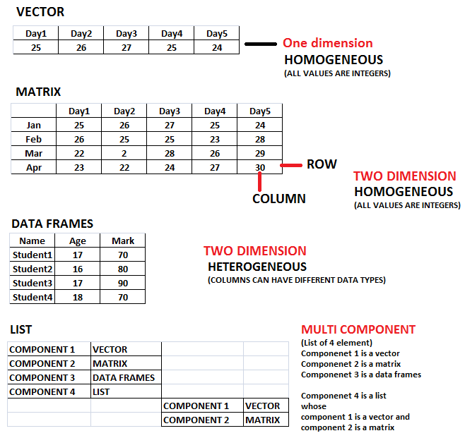
Figure 1: Data structures in R

2.9 Vector

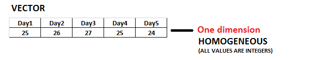
Figure 1: Vector

Vector is one dimensional way of data storage in which sequence of numbers/characters/logical values can be stored. In the above image, example shows measured temperature of a city for 5 days. So we have 5 temperature values and all values are of integer type (25C, 30C etc). These 5 integers are stored in a sequence, which we term as integer vector (A vector storing integers). Therefore a vector can be understood as a single entity/variable/object storing an ordered collection of elements. Similarly, names of each students in a class can be stored in the form of a Character vector. Since all elements stored in a vector are of only one data types, i.e either integer or numeric or character or logical, vector is a homogeneous data structure (integer vector, numeric vector, character vector and logical vector respectively).

2.9.1 Creating a vector

In R vectors can be created using

Assignment operator (=)
Range operator (:)
Concatenate function c()
Sequence function seq()
Repeat function rep()
Sample function

We will explore these one by one.

2.9.2 Create Vector of one element

x1=2; # Integer data type
x2=2.3; # Numeric data type
x3="A"; # Single Character. Double quote was used.
x4="ABC"; # Multiple Characters. Double quote was used.
x5='A'; # Single Character. Single quote was used.
x6='ABC'; # Multiple Characters. Single quote was used.
x7=TRUE; # Logical. Note the use of TRUE (All capital)
x8=FALSE; # Logical. Note the use of FALSE (All capital)
#x9=true;  # Error since true is written in small. R is case sensitive.

In the above examples, x1 is an integer vector of one element having value 2. Similarly x2 is a numeric vector with one element 2.3. The vectors x3, x4, x5 and x6 are character vectors storing character data. Note that the character data can be either single character (“A”) or multiple character (“ABC”). Similarly one can use either single or double quote to assign character data types. The vector x7 and x8 are logical vector storing boolean values (TRUE or FALSE). Note that TRUE/FALSE can be also be written as T/F but everything has to be capital. R is case sensitive i.e. X and x are different. Thus x9=true; will throw error since R will not understand true.
The = is assignment operator using which the results from right hand side expression is stored in left hand side variable. When we say x1=2, 2 (right side) is assigned to x1 (left side).
Also note semicolon (;) at the end of few statements. Use of ; is optional. However it is recommended that you must end every statement with ; so that R understands it is end of a statement.

So far we saw vectors with one element. Now we will explore how to create vectors with more than one element.

2.9.3 Create Vector using Range operator (:)

x1=1:5; 
x1;

## [1] 1 2 3 4 5

x2=5:1;
x2;

## [1] 5 4 3 2 1

In the above example x1 stores 5 elements 1, 2, 3, 4 and 5 while x2 stores 5, 4, 3, 2, 1. So using range operator you can assign more than one element incremented/decremented by 1.

2.9.4 Create Vector using c()

Range operator (:) is handy when you have sequence of integers incremented or decremented by 1. What if you have random data and there is no pattern. In such case you can use concatenate function c().

# Integer vector with 3 element
x1=c(2,10,35);
x1;

## [1]  2 10 35

# Character vector with 3 elements
x2=c("Gene","Expression",'Chromosome');
x2;

## [1] "Gene"       "Expression" "Chromosome"

# Logical vector
x3=c(T,F,TRUE,FALSE);
x3;

## [1]  TRUE FALSE  TRUE FALSE

x4=c(x1,44,55);  # x4 will now contain 2, 10, 35, 44, 55
x4;

## [1]  2 10 35 44 55

In the example x1 is a vector with 3 elements: 2, 10 and 35. Similarly x2 is a character vector and x3 is a logical vector. Note that, since x2 is a character vector and each element are characters, you have to write within either single or double quote (e.g. “Gene”, “Expression”, ‘Chromosome’). In case of x4, first element is x1 vector thus x4 will first store 2, 10, 35 followed by 44 and 55.

2.9.5 seq() function

Generate regular sequences using seq() function.

# Generate a sequence of number from 0 to 10 incremented by 2
x1=seq(from=0, to=10, by=2)
x1;

## [1]  0  2  4  6  8 10

# Generate a sequence of 50 number from 0 to 10
x2=seq(from=0, to=10, length=30)
x2;

##  [1]  0.0000000  0.3448276  0.6896552  1.0344828  1.3793103  1.7241379
##  [7]  2.0689655  2.4137931  2.7586207  3.1034483  3.4482759  3.7931034
## [13]  4.1379310  4.4827586  4.8275862  5.1724138  5.5172414  5.8620690
## [19]  6.2068966  6.5517241  6.8965517  7.2413793  7.5862069  7.9310345
## [25]  8.2758621  8.6206897  8.9655172  9.3103448  9.6551724 10.0000000

In R there are several inbuilt functions which can be used to do certain tasks. Functions can be called by their name followed by (). Inside () various parameters required to the function can be passed as key=value pair. In the above example to x1 will generate sequence of number from 0 (from=0) to 10 (to=10), incremented by 2 (by=2). Thus x2 will contain 0, 2, 4, 6, 8 and 10. Note that from=0, to=10 and by=2 are 3 parameters which we pass to seq() function and these are separated by comma (,). In case of 2nd example, we just replace by parameter with length=50. So we use same function to generate 50 elements between 0 to 10.

2.9.6 rep() function

rep replicates the values in x.

# Create a vector x1 with 3 elements
x1=c(2,3,5);
x1;

## [1] 2 3 5

# Repeat each element of x1, 3 times
x2=rep(x1,each=3);
x2;

## [1] 2 2 2 3 3 3 5 5 5

# Repeat x1, 3 times.
x3=rep(x1, times=3);
x3;

## [1] 2 3 5 2 3 5 2 3 5

rep(1:4, each = 2, times = 4);

##  [1] 1 1 2 2 3 3 4 4 1 1 2 2 3 3 4 4 1 1 2 2 3 3 4 4 1 1 2 2 3 3 4 4

x1 is a vector with 3 elements (2, 3, 5). Using rep() function, the first argument we pass is a vector, when we specify each=3, rep() function will repeat each element of x1 3 times and store in x2. Thus x2 will store 2, 2, 2, 3, 3, 3, 5, 5, 5. When we specify times=3, rep() function will repeat the x1 vector 3 times. Thus x3 will store 2, 3, 5, 2, 3, 5, 2, 3, 5.

2.9.7 sample() function

sample takes a sample of the specified size from the elements of x using either with or without replacement.

# Fetch 10 random number from the database 1:50
sample(1:50, 10);

##  [1] 23  6 13 14 32 48 30 21 35 44

# Fetch 100 random number from the database 20:30. Since we are fetching more elements than present in database, we need to specify replace=TRUE (Should sampling be with replacement?)
sample(20:30, 100, replace = TRUE);

##   [1] 23 28 29 26 30 28 20 22 25 22 28 21 23 20 30 29 27 27 20 30 20 27 30
##  [24] 29 28 24 28 29 25 28 30 22 25 22 25 29 27 23 23 27 30 24 25 25 21 23
##  [47] 20 20 24 21 30 24 28 23 22 20 24 28 30 27 21 22 30 29 23 30 20 27 26
##  [70] 30 25 27 27 22 27 30 26 26 23 25 26 27 27 21 29 26 28 25 30 28 23 25
##  [93] 30 30 20 23 22 22 25 24

2.9.8 rnorm() function

The Normal Distribution.

# Fetch 50 element from a normal distribution
rnorm(50);

##  [1]  0.1072768 -0.5559458 -0.9473100  0.1231852 -0.4192404  0.6580416
##  [7]  0.2922227 -1.3781758 -0.4989867 -0.3913664  0.4577026 -0.6573956
## [13] -0.2745708 -1.5240526 -0.1586570  0.7814693  0.2665822  0.6159602
## [19] -0.7086050  1.4935373 -0.7845990 -0.6681351  0.1259791 -0.7627799
## [25] -2.3429657  0.4638053 -0.9005353 -0.1291929  1.4176135 -1.6138372
## [31]  1.9607997 -0.1071785  1.3359480  0.6585954  0.4056754 -1.4911310
## [37] -0.6782876 -0.9751761  0.4949637  2.0767209 -0.7519678  0.4856761
## [43]  0.1120740  0.7585012  0.7791965 -0.9262399 -1.4125175  1.0071076
## [49] -0.2031515 -0.3368814

rnorm(50, mean=5, sd=2);

##  [1]  7.625584  8.340640  4.248128  4.073515  6.697424  4.330564  3.905983
##  [8] -3.074845  3.286376  5.482962  6.590412  4.316969  7.530495  4.821459
## [15]  6.100846  5.019444  4.324496  5.395754  5.443038  5.380750  5.860219
## [22]  1.380844  5.849956  8.782875  2.359652  6.724360  2.148440  5.552696
## [29]  5.075265  5.183448  5.150578  4.746253  4.567021  4.905083  6.280027
## [36]  4.618495  6.076839  3.244405  2.279278  7.211379  6.265323  4.911341
## [43]  7.447383  7.235156  3.536407  4.521768  3.954108  3.551843  4.229697
## [50]  6.761596

Task: Now Go to Task page and finish Vector creation

2.9.9 Fetching elements from a vector

x=c(10,20,30,40,50,60);
length(x);

## [1] 6

x[1]; # 1st element

## [1] 10

x[4]; # 4th element

## [1] 40

x[2:3]; # 2nd to 3rd element

## [1] 20 30

x[c(1,3,5)]; # 1st, 3rd, 4th element

## [1] 10 30 50

x[3:length(x)];

## [1] 30 40 50 60

x[-1]; # Exclude 1st element

## [1] 20 30 40 50 60

x[-c(1,3)] # Exclude 1st, 3rd element

## [1] 20 40 50 60

x[10]; # NA: Missing value

## [1] NA

# x[1, 3, 5] # Error

2.9.10 Delete element(s) from a vector

x=10:20;
x;

##  [1] 10 11 12 13 14 15 16 17 18 19 20

x=x[-3];
x;

##  [1] 10 11 13 14 15 16 17 18 19 20

x=x[-c(7,3)];
x;

## [1] 10 11 14 15 16 18 19 20

x=x[-c(2,length(x))];
x;

## [1] 10 14 15 16 18 19

2.9.11 Add element(s) to existing vector

x=10:20;
x;

##  [1] 10 11 12 13 14 15 16 17 18 19 20

x=c(x,55);
x;

##  [1] 10 11 12 13 14 15 16 17 18 19 20 55

x=c(33,x,77);
x;

##  [1] 33 10 11 12 13 14 15 16 17 18 19 20 55 77

y=seq(100,110,0.5);
y;

##  [1] 100.0 100.5 101.0 101.5 102.0 102.5 103.0 103.5 104.0 104.5 105.0
## [12] 105.5 106.0 106.5 107.0 107.5 108.0 108.5 109.0 109.5 110.0

x=c(x,y);
x;

##  [1]  33.0  10.0  11.0  12.0  13.0  14.0  15.0  16.0  17.0  18.0  19.0
## [12]  20.0  55.0  77.0 100.0 100.5 101.0 101.5 102.0 102.5 103.0 103.5
## [23] 104.0 104.5 105.0 105.5 106.0 106.5 107.0 107.5 108.0 108.5 109.0
## [34] 109.5 110.0

2.9.12 Replace elements in existing vector

x=sample(20:30, 5);
x;

## [1] 24 23 29 22 25

x[2]=111111;
x;

## [1]     24 111111     29     22     25

x[c(1,3)]=c(555, 777);
x;

## [1]    555 111111    777     22     25

Task: Now Go to Task page and finish Fetching vector elements and Vector manipulation section

2.9.13 Inbuilt functions for numeric vector

x=seq(4, 8, length=10);
x;

##  [1] 4.000000 4.444444 4.888889 5.333333 5.777778 6.222222 6.666667
##  [8] 7.111111 7.555556 8.000000

length(x);

## [1] 10

sort(x);

##  [1] 4.000000 4.444444 4.888889 5.333333 5.777778 6.222222 6.666667
##  [8] 7.111111 7.555556 8.000000

order(x);

##  [1]  1  2  3  4  5  6  7  8  9 10

max(x);

## [1] 8

min(x);

## [1] 4

range(x);

## [1] 4 8

mean(x);

## [1] 6

median(x);

## [1] 6

mode(x);

## [1] "numeric"

sd(x);

## [1] 1.345622

var(x);

## [1] 1.8107

quantile(x);

##   0%  25%  50%  75% 100% 
##    4    5    6    7    8

summary(x);

##    Min. 1st Qu.  Median    Mean 3rd Qu.    Max. 
##       4       5       6       6       7       8

sin(x);

##  [1] -0.75680250 -0.96431712 -0.98446429 -0.81332939 -0.48416406
##  [6] -0.06092533  0.37415123  0.73652996  0.95580043  0.98935825

log(x, base=2);

##  [1] 2.000000 2.152003 2.289507 2.415037 2.530515 2.637430 2.736966
##  [8] 2.830075 2.917538 3.000000

log(x, base=10);

##  [1] 0.6020600 0.6478175 0.6892102 0.7269987 0.7617608 0.7939455 0.8239087
##  [8] 0.8519375 0.8782664 0.9030900

2.9.14 Correlation using cor()

x=sample(1:100,20);
y=sample(1:100,20);
x;

##  [1] 69 75  7 33 53 48 43 76 70 79 34 92 49 95 26 57 21 62 40 60

y;

##  [1] 71 92 20 78  6  3 68  2 35 26  8 87 51 91 16 55 84 85 32 38

# Methods: "pearson", "kendall", "spearman"
cor(x,y, method = "spearman");

## [1] 0.3022556

cor(x,y, method = "pearson");

## [1] 0.3083698

2.9.15 Set operations

x;

##  [1] 69 75  7 33 53 48 43 76 70 79 34 92 49 95 26 57 21 62 40 60

y;

##  [1] 71 92 20 78  6  3 68  2 35 26  8 87 51 91 16 55 84 85 32 38

union(x,y);

##  [1] 69 75  7 33 53 48 43 76 70 79 34 92 49 95 26 57 21 62 40 60 71 20 78
## [24]  6  3 68  2 35  8 87 51 91 16 55 84 85 32 38

intersect(x,y);

## [1] 92 26

setdiff(x,y); # x - y

##  [1] 69 75  7 33 53 48 43 76 70 79 34 49 95 57 21 62 40 60

setdiff(y,x); # y - x

##  [1] 71 20 78  6  3 68  2 35  8 87 51 91 16 55 84 85 32 38

2.9.16 Arithmetic expressions

Vector recycling. Shorter vector are recycled to match the length of longest vector. Once length of all vectors are equal, then arithmentic operations are performed.

x=c(3,4,5,6);
y=c(6,7,8,9);
z=c(1,2);
p=c(9,10,11);
x+y;

## [1]  9 11 13 15

x+z;

## [1] 4 6 6 8

x+p;

## Warning in x + p: longer object length is not a multiple of shorter object
## length

## [1] 12 14 16 15

2.9.17 Arithmetic operations on vector

x=1:3;
y=6:8;
z=10:12;
x;

## [1] 1 2 3

y;

## [1] 6 7 8

z;

## [1] 10 11 12

x-y;

## [1] -5 -5 -5

x*4;

## [1]  4  8 12

x*y;

## [1]  6 14 24

y/5;

## [1] 1.2 1.4 1.6

y%%5;

## [1] 1 2 3

y^3;

## [1] 216 343 512

2.9.18 Operator precedence

x+2*y+z;

## [1] 23 27 31

x+2*y/z;

## [1] 2.200000 3.272727 4.333333

(x+2)*y+z;

## [1] 28 39 52

(x+2)*(y+z);

## [1]  48  72 100

n=10;
1:n-1;

##  [1] 0 1 2 3 4 5 6 7 8 9

1:(n-1);

## [1] 1 2 3 4 5 6 7 8 9

Task: Now Go to Task page and finish Vector arithmetic

2.9.19 Conditional statements

x=10:30;
x;

##  [1] 10 11 12 13 14 15 16 17 18 19 20 21 22 23 24 25 26 27 28 29 30

x > 15;

##  [1] FALSE FALSE FALSE FALSE FALSE FALSE  TRUE  TRUE  TRUE  TRUE  TRUE
## [12]  TRUE  TRUE  TRUE  TRUE  TRUE  TRUE  TRUE  TRUE  TRUE  TRUE

x == 15;

##  [1] FALSE FALSE FALSE FALSE FALSE  TRUE FALSE FALSE FALSE FALSE FALSE
## [12] FALSE FALSE FALSE FALSE FALSE FALSE FALSE FALSE FALSE FALSE

x > 15 & x %% 2==0;

##  [1] FALSE FALSE FALSE FALSE FALSE FALSE  TRUE FALSE  TRUE FALSE  TRUE
## [12] FALSE  TRUE FALSE  TRUE FALSE  TRUE FALSE  TRUE FALSE  TRUE

x[x > 15 & x %% 2==0];

## [1] 16 18 20 22 24 26 28 30

x > 15 | x %% 2==0;

##  [1]  TRUE FALSE  TRUE FALSE  TRUE FALSE  TRUE  TRUE  TRUE  TRUE  TRUE
## [12]  TRUE  TRUE  TRUE  TRUE  TRUE  TRUE  TRUE  TRUE  TRUE  TRUE

x[x > 15 | x %% 2==0];

##  [1] 10 12 14 16 17 18 19 20 21 22 23 24 25 26 27 28 29 30

# which() function returns the indices which satisfies the condition to TRUE
tempind=which(x > 15 & x %% 2==0);
tempind;

## [1]  7  9 11 13 15 17 19 21

x[tempind];

## [1] 16 18 20 22 24 26 28 30

2.9.20 Check for missing values

x=c(1:5,NA,NA,2:3,NA,NA,3);
is.na(x);

##  [1] FALSE FALSE FALSE FALSE FALSE  TRUE  TRUE FALSE FALSE  TRUE  TRUE
## [12] FALSE

which(is.na(x));

## [1]  6  7 10 11

2.9.21 Check data types and data structures

x1=1:10;
str(x1);

##  int [1:10] 1 2 3 4 5 6 7 8 9 10

x2=c(1.2, 2.3);
str(x2);

##  num [1:2] 1.2 2.3

x3=c("aaa","bbb");
str(x3);

##  chr [1:2] "aaa" "bbb"

x4=c('ccc','ddd');
str(x4);

##  chr [1:2] "ccc" "ddd"

x5=c(T,F);
str(x5);

##  logi [1:2] TRUE FALSE

str(letters);

##  chr [1:26] "a" "b" "c" "d" "e" "f" "g" "h" "i" "j" "k" "l" "m" "n" ...

2.9.22 Implicit Data type conversion

Conversion Order: Logical -> Integer -> Numeric -> character

x1=c(1, "abc", TRUE);
str(x1);

##  chr [1:3] "1" "abc" "TRUE"

x2=c(1,TRUE);
str(x2);

##  num [1:2] 1 1

2.9.23 Character vector and related functions

x=c("gene1","gene2","gene3");
y=c('prot','rna','lipid');
z=letters;
nchar(x);

## [1] 5 5 5

nchar(y);

## [1] 4 3 5

substr("abcdef", 2, 4);

## [1] "bcd"

substr(c(x,y), 1, 2);

## [1] "ge" "ge" "ge" "pr" "rn" "li"

paste(letters, 1:5);

##  [1] "a 1" "b 2" "c 3" "d 4" "e 5" "f 1" "g 2" "h 3" "i 4" "j 5" "k 1"
## [12] "l 2" "m 3" "n 4" "o 5" "p 1" "q 2" "r 3" "s 4" "t 5" "u 1" "v 2"
## [23] "w 3" "x 4" "y 5" "z 1"

paste(letters, 1:5, sep=":");

##  [1] "a:1" "b:2" "c:3" "d:4" "e:5" "f:1" "g:2" "h:3" "i:4" "j:5" "k:1"
## [12] "l:2" "m:3" "n:4" "o:5" "p:1" "q:2" "r:3" "s:4" "t:5" "u:1" "v:2"
## [23] "w:3" "x:4" "y:5" "z:1"

paste(letters, 1:5, sep=":", collapse = ",");

## [1] "a:1,b:2,c:3,d:4,e:5,f:1,g:2,h:3,i:4,j:5,k:1,l:2,m:3,n:4,o:5,p:1,q:2,r:3,s:4,t:5,u:1,v:2,w:3,x:4,y:5,z:1"

2.9.24 Explicit Data Type Conversion

x=c("1","2","3");
str(x);

##  chr [1:3] "1" "2" "3"

x=as.numeric(x);
str(x);

##  num [1:3] 1 2 3

x=1:5;
str(x);

##  int [1:5] 1 2 3 4 5

x=as.character(x);
str(x);

##  chr [1:5] "1" "2" "3" "4" "5"

2.10 Matrix

2.10.1 Create a matrix from vector using dim attributes

x=21:70;
dim(x)=c(10,5); # 10 row, 5 col
x;

##       [,1] [,2] [,3] [,4] [,5]
##  [1,]   21   31   41   51   61
##  [2,]   22   32   42   52   62
##  [3,]   23   33   43   53   63
##  [4,]   24   34   44   54   64
##  [5,]   25   35   45   55   65
##  [6,]   26   36   46   56   66
##  [7,]   27   37   47   57   67
##  [8,]   28   38   48   58   68
##  [9,]   29   39   49   59   69
## [10,]   30   40   50   60   70

2.10.2 Create matrix using matrix()

x=21:70;
matrix(x, ncol=10); # 10 col

##      [,1] [,2] [,3] [,4] [,5] [,6] [,7] [,8] [,9] [,10]
## [1,]   21   26   31   36   41   46   51   56   61    66
## [2,]   22   27   32   37   42   47   52   57   62    67
## [3,]   23   28   33   38   43   48   53   58   63    68
## [4,]   24   29   34   39   44   49   54   59   64    69
## [5,]   25   30   35   40   45   50   55   60   65    70

m=matrix(x, ncol=10, byrow = TRUE); # Fill elements row wise

2.10.3 Functions that can be applied to a matrix

# Data structure of m
str(m);

##  int [1:5, 1:10] 21 31 41 51 61 22 32 42 52 62 ...

# Dimension of m
dim(m);

## [1]  5 10

# Number of rows
nrow(m);

## [1] 5

# Number of columns
ncol(m);

## [1] 10

# Column means
colMeans(m);

##  [1] 41 42 43 44 45 46 47 48 49 50

# Row means
rowMeans(m);

## [1] 25.5 35.5 45.5 55.5 65.5

# Transpose
t(m);

##       [,1] [,2] [,3] [,4] [,5]
##  [1,]   21   31   41   51   61
##  [2,]   22   32   42   52   62
##  [3,]   23   33   43   53   63
##  [4,]   24   34   44   54   64
##  [5,]   25   35   45   55   65
##  [6,]   26   36   46   56   66
##  [7,]   27   37   47   57   67
##  [8,]   28   38   48   58   68
##  [9,]   29   39   49   59   69
## [10,]   30   40   50   60   70

# Fetch column names
colnames(m);

## NULL

# Fetch row names
rownames(m);

## NULL

# head
head(m);

##      [,1] [,2] [,3] [,4] [,5] [,6] [,7] [,8] [,9] [,10]
## [1,]   21   22   23   24   25   26   27   28   29    30
## [2,]   31   32   33   34   35   36   37   38   39    40
## [3,]   41   42   43   44   45   46   47   48   49    50
## [4,]   51   52   53   54   55   56   57   58   59    60
## [5,]   61   62   63   64   65   66   67   68   69    70

2.10.4 Assign column/row names

colnames(m)=paste("C",1:ncol(m),sep="");
rownames(m)=paste("R",1:nrow(m),sep="");
m;

##    C1 C2 C3 C4 C5 C6 C7 C8 C9 C10
## R1 21 22 23 24 25 26 27 28 29  30
## R2 31 32 33 34 35 36 37 38 39  40
## R3 41 42 43 44 45 46 47 48 49  50
## R4 51 52 53 54 55 56 57 58 59  60
## R5 61 62 63 64 65 66 67 68 69  70

2.10.5 Fetch elements from a matrix using indices

m;

##    C1 C2 C3 C4 C5 C6 C7 C8 C9 C10
## R1 21 22 23 24 25 26 27 28 29  30
## R2 31 32 33 34 35 36 37 38 39  40
## R3 41 42 43 44 45 46 47 48 49  50
## R4 51 52 53 54 55 56 57 58 59  60
## R5 61 62 63 64 65 66 67 68 69  70

# 1st row, 3rd column
m[1,3];

## [1] 23

# 1st tp 3rd row and 3rd to 5th column
m[c(1:3),c(3:5)];

##    C3 C4 C5
## R1 23 24 25
## R2 33 34 35
## R3 43 44 45

# 1st row
m[1,];

##  C1  C2  C3  C4  C5  C6  C7  C8  C9 C10 
##  21  22  23  24  25  26  27  28  29  30

# 3rd column
m[,3];

## R1 R2 R3 R4 R5 
## 23 33 43 53 63

# 3rd element. Here matrix is converted to vector and 3rd element is returned
m[3];

## [1] 41

2.10.6 Fetch element using index matrix

m;

##    C1 C2 C3 C4 C5 C6 C7 C8 C9 C10
## R1 21 22 23 24 25 26 27 28 29  30
## R2 31 32 33 34 35 36 37 38 39  40
## R3 41 42 43 44 45 46 47 48 49  50
## R4 51 52 53 54 55 56 57 58 59  60
## R5 61 62 63 64 65 66 67 68 69  70

index=c(2,3,3,4,4,5);
m[index]

## [1] 31 41 41 51 51 61

2.10.7 Fetch elements from a matrix using row and column names

m;

##    C1 C2 C3 C4 C5 C6 C7 C8 C9 C10
## R1 21 22 23 24 25 26 27 28 29  30
## R2 31 32 33 34 35 36 37 38 39  40
## R3 41 42 43 44 45 46 47 48 49  50
## R4 51 52 53 54 55 56 57 58 59  60
## R5 61 62 63 64 65 66 67 68 69  70

m["R1","C3"];

## [1] 23

2.10.8 Insert rows and columns by rbind() and cbind()

m1=matrix(1:10, nrow=5);
m1;

##      [,1] [,2]
## [1,]    1    6
## [2,]    2    7
## [3,]    3    8
## [4,]    4    9
## [5,]    5   10

m1=rbind(m1, 999);
m1;

##      [,1] [,2]
## [1,]    1    6
## [2,]    2    7
## [3,]    3    8
## [4,]    4    9
## [5,]    5   10
## [6,]  999  999

m1=rbind(m1, c(2,3));
m1;

##      [,1] [,2]
## [1,]    1    6
## [2,]    2    7
## [3,]    3    8
## [4,]    4    9
## [5,]    5   10
## [6,]  999  999
## [7,]    2    3

m1=cbind(m1, 1:5);

## Warning in cbind(m1, 1:5): number of rows of result is not a multiple of
## vector length (arg 2)

m1;

##      [,1] [,2] [,3]
## [1,]    1    6    1
## [2,]    2    7    2
## [3,]    3    8    3
## [4,]    4    9    4
## [5,]    5   10    5
## [6,]  999  999    1
## [7,]    2    3    2

m1=cbind(m1, 10:20);

## Warning in cbind(m1, 10:20): number of rows of result is not a multiple of
## vector length (arg 2)

m1;

##      [,1] [,2] [,3] [,4]
## [1,]    1    6    1   10
## [2,]    2    7    2   11
## [3,]    3    8    3   12
## [4,]    4    9    4   13
## [5,]    5   10    5   14
## [6,]  999  999    1   15
## [7,]    2    3    2   16

2.10.9 Create matrix using rbind() and cbind()

x=seq(2, 4, length=10);
y=1:10;
x;

##  [1] 2.000000 2.222222 2.444444 2.666667 2.888889 3.111111 3.333333
##  [8] 3.555556 3.777778 4.000000

y;

##  [1]  1  2  3  4  5  6  7  8  9 10

cbind(x,y);

##              x  y
##  [1,] 2.000000  1
##  [2,] 2.222222  2
##  [3,] 2.444444  3
##  [4,] 2.666667  4
##  [5,] 2.888889  5
##  [6,] 3.111111  6
##  [7,] 3.333333  7
##  [8,] 3.555556  8
##  [9,] 3.777778  9
## [10,] 4.000000 10

rbind(x,y);

##   [,1]     [,2]     [,3]     [,4]     [,5]     [,6]     [,7]     [,8]
## x    2 2.222222 2.444444 2.666667 2.888889 3.111111 3.333333 3.555556
## y    1 2.000000 3.000000 4.000000 5.000000 6.000000 7.000000 8.000000
##       [,9] [,10]
## x 3.777778     4
## y 9.000000    10

2.10.10 Delete row(s) and column(s)

m;

##    C1 C2 C3 C4 C5 C6 C7 C8 C9 C10
## R1 21 22 23 24 25 26 27 28 29  30
## R2 31 32 33 34 35 36 37 38 39  40
## R3 41 42 43 44 45 46 47 48 49  50
## R4 51 52 53 54 55 56 57 58 59  60
## R5 61 62 63 64 65 66 67 68 69  70

m=m[-1,];
m;

##    C1 C2 C3 C4 C5 C6 C7 C8 C9 C10
## R2 31 32 33 34 35 36 37 38 39  40
## R3 41 42 43 44 45 46 47 48 49  50
## R4 51 52 53 54 55 56 57 58 59  60
## R5 61 62 63 64 65 66 67 68 69  70

m=m[,-3];
m;

##    C1 C2 C4 C5 C6 C7 C8 C9 C10
## R2 31 32 34 35 36 37 38 39  40
## R3 41 42 44 45 46 47 48 49  50
## R4 51 52 54 55 56 57 58 59  60
## R5 61 62 64 65 66 67 68 69  70

2.10.11 Check for matrix

is.matrix(m);

## [1] TRUE

2.10.12 Conditional statements on matrix

m;

##    C1 C2 C4 C5 C6 C7 C8 C9 C10
## R2 31 32 34 35 36 37 38 39  40
## R3 41 42 44 45 46 47 48 49  50
## R4 51 52 54 55 56 57 58 59  60
## R5 61 62 64 65 66 67 68 69  70

m%%5==0;

##       C1    C2    C4   C5    C6    C7    C8    C9  C10
## R2 FALSE FALSE FALSE TRUE FALSE FALSE FALSE FALSE TRUE
## R3 FALSE FALSE FALSE TRUE FALSE FALSE FALSE FALSE TRUE
## R4 FALSE FALSE FALSE TRUE FALSE FALSE FALSE FALSE TRUE
## R5 FALSE FALSE FALSE TRUE FALSE FALSE FALSE FALSE TRUE

which(m%%5==0, arr.ind = TRUE);

##    row col
## R2   1   4
## R3   2   4
## R4   3   4
## R5   4   4
## R2   1   9
## R3   2   9
## R4   3   9
## R5   4   9

Task: Now Go to Task page and finish Matrix

2.11 Data Frame

2.11.1 Create a data frame

x=1:26;
z=letters;
y=paste(z, x, sep=":");
d=data.frame(C1=x, C2=y, C3=z);
d;

##    C1   C2 C3
## 1   1  a:1  a
## 2   2  b:2  b
## 3   3  c:3  c
## 4   4  d:4  d
## 5   5  e:5  e
## 6   6  f:6  f
## 7   7  g:7  g
## 8   8  h:8  h
## 9   9  i:9  i
## 10 10 j:10  j
## 11 11 k:11  k
## 12 12 l:12  l
## 13 13 m:13  m
## 14 14 n:14  n
## 15 15 o:15  o
## 16 16 p:16  p
## 17 17 q:17  q
## 18 18 r:18  r
## 19 19 s:19  s
## 20 20 t:20  t
## 21 21 u:21  u
## 22 22 v:22  v
## 23 23 w:23  w
## 24 24 x:24  x
## 25 25 y:25  y
## 26 26 z:26  z

str(d);

## 'data.frame':    26 obs. of  3 variables:
##  $ C1: int  1 2 3 4 5 6 7 8 9 10 ...
##  $ C2: Factor w/ 26 levels "a:1","b:2","c:3",..: 1 2 3 4 5 6 7 8 9 10 ...
##  $ C3: Factor w/ 26 levels "a","b","c","d",..: 1 2 3 4 5 6 7 8 9 10 ...

colnames(d);

## [1] "C1" "C2" "C3"

rownames(d);

##  [1] "1"  "2"  "3"  "4"  "5"  "6"  "7"  "8"  "9"  "10" "11" "12" "13" "14"
## [15] "15" "16" "17" "18" "19" "20" "21" "22" "23" "24" "25" "26"

dim(d);

## [1] 26  3

# edit(d);

2.11.2 Fetch values from a data frame

d;

##    C1   C2 C3
## 1   1  a:1  a
## 2   2  b:2  b
## 3   3  c:3  c
## 4   4  d:4  d
## 5   5  e:5  e
## 6   6  f:6  f
## 7   7  g:7  g
## 8   8  h:8  h
## 9   9  i:9  i
## 10 10 j:10  j
## 11 11 k:11  k
## 12 12 l:12  l
## 13 13 m:13  m
## 14 14 n:14  n
## 15 15 o:15  o
## 16 16 p:16  p
## 17 17 q:17  q
## 18 18 r:18  r
## 19 19 s:19  s
## 20 20 t:20  t
## 21 21 u:21  u
## 22 22 v:22  v
## 23 23 w:23  w
## 24 24 x:24  x
## 25 25 y:25  y
## 26 26 z:26  z

d[,1];

##  [1]  1  2  3  4  5  6  7  8  9 10 11 12 13 14 15 16 17 18 19 20 21 22 23
## [24] 24 25 26

d$C1;

##  [1]  1  2  3  4  5  6  7  8  9 10 11 12 13 14 15 16 17 18 19 20 21 22 23
## [24] 24 25 26

d[3,];

##   C1  C2 C3
## 3  3 c:3  c

d[3,1];

## [1] 3

d$C1[3];

## [1] 3

2.11.3 Insert column to data frame

d;

##    C1   C2 C3
## 1   1  a:1  a
## 2   2  b:2  b
## 3   3  c:3  c
## 4   4  d:4  d
## 5   5  e:5  e
## 6   6  f:6  f
## 7   7  g:7  g
## 8   8  h:8  h
## 9   9  i:9  i
## 10 10 j:10  j
## 11 11 k:11  k
## 12 12 l:12  l
## 13 13 m:13  m
## 14 14 n:14  n
## 15 15 o:15  o
## 16 16 p:16  p
## 17 17 q:17  q
## 18 18 r:18  r
## 19 19 s:19  s
## 20 20 t:20  t
## 21 21 u:21  u
## 22 22 v:22  v
## 23 23 w:23  w
## 24 24 x:24  x
## 25 25 y:25  y
## 26 26 z:26  z

d$C5=1;
# d$C6=1:100; #Error
d$C6=seq(3, 8, length=26);

2.11.4 Delete column or row from data frame

d$C5=NULL;
head(d);

##   C1  C2 C3  C6
## 1  1 a:1  a 3.0
## 2  2 b:2  b 3.2
## 3  3 c:3  c 3.4
## 4  4 d:4  d 3.6
## 5  5 e:5  e 3.8
## 6  6 f:6  f 4.0

2.11.5 Check for data frame

is.data.frame(d);

## [1] TRUE

Task: Now Go to Task page and finish Data Frame

2.12 List

An R list is an object consisting of an ordered collection of objects known as its components.

x1=1:5; # vector
x2=matrix(1:20, ncol=5);
x3= data.frame(1:5, letters[1:5]);
mylist = list(comp1=x1, comp2=x2, comp3=x3);
mylist;

## $comp1
## [1] 1 2 3 4 5
## 
## $comp2
##      [,1] [,2] [,3] [,4] [,5]
## [1,]    1    5    9   13   17
## [2,]    2    6   10   14   18
## [3,]    3    7   11   15   19
## [4,]    4    8   12   16   20
## 
## $comp3
##   X1.5 letters.1.5.
## 1    1            a
## 2    2            b
## 3    3            c
## 4    4            d
## 5    5            e

2.12.1 Access component of list using $ notation

# Access componene1 using $ notation
mylist$comp1;

## [1] 1 2 3 4 5

mylist$comp2;

##      [,1] [,2] [,3] [,4] [,5]
## [1,]    1    5    9   13   17
## [2,]    2    6   10   14   18
## [3,]    3    7   11   15   19
## [4,]    4    8   12   16   20

2.12.2 Access component of list using []

Using [] returns list while using [[]] returns the component.

# Fetching 2nd component using []. Returns list
m1 = mylist[2];
# Fetching 2nd component using [[]]. Returns matrix
m2 = mylist[[2]];
m1;

## $comp2
##      [,1] [,2] [,3] [,4] [,5]
## [1,]    1    5    9   13   17
## [2,]    2    6   10   14   18
## [3,]    3    7   11   15   19
## [4,]    4    8   12   16   20

str(m1);

## List of 1
##  $ comp2: int [1:4, 1:5] 1 2 3 4 5 6 7 8 9 10 ...

m2;

##      [,1] [,2] [,3] [,4] [,5]
## [1,]    1    5    9   13   17
## [2,]    2    6   10   14   18
## [3,]    3    7   11   15   19
## [4,]    4    8   12   16   20

str(m2);

##  int [1:4, 1:5] 1 2 3 4 5 6 7 8 9 10 ...