Chapter 7 R Case study and Tasks

7.1 Case study1: Gene Expression Data Analysis

7.1.1 Experimental setup

There are two varieties of plant xyz, one is resistant (R) to a fungal infection while other is susceptible to the fungal disease (D). The experiment was conducted to study the differential expression of 490 genes (G1, G2, G3,.., G490), which are involved in 3 different pathways (P1, P2 and P3).

The gene expression was measured in the two mentioned varieties of plants, R and D, on Day 2, Day 4, Day 6 and Day 8.

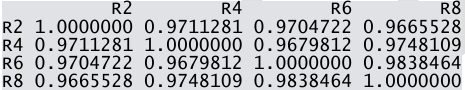
The gene expression values for variety R on these days are given as R2, R4, R6 and R8 and that for variety D are given as D2, D4, D6 and D8.

The gene expression data is stored in a file path.txt. The first 6 rows of the file are shown below.

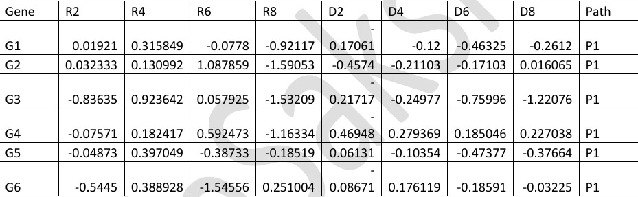
7.1.2 Objective

Data exploration, visualization and analysis of gene expression data, in a given file, using R to find out those genes, which are differentially expressed on 3 or more days between two varieties, R and D.

7.1.3 Steps

1. Import the file “path.txt” into R.
2. What is the data structure of imported file?
3. How many rows and columns are there?
4. What are column names?
5. Find out minimum, first quantile, median, third quantile, mean and maximum of expression values on each day. Store the result in a file.
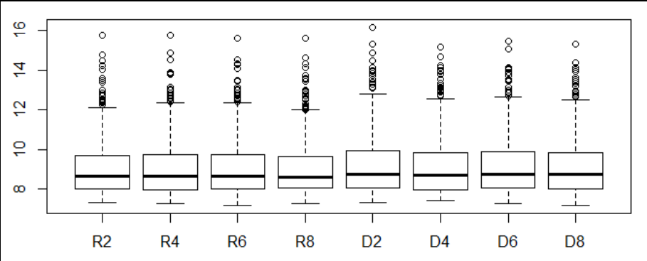
6. Visualization of gene expression on 2,4,6,8 days of D and R plants using boxplot.

7.1.3.1 .

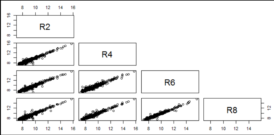
7. Visualization of pairwise correlation of gene expressions among R2, R4, R6 and R8.

7.1.3.2 .

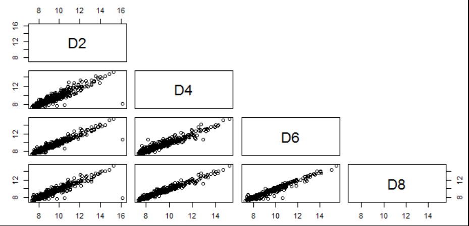
8. Visualization of pairwise correlation of gene expressions among D2, D4, D6 and D8.

7.1.3.3 .

9. Calculate the pairwise correlation coefficient values among R2, R4, R6 and R8.

7.1.3.4 .

10. Calculate the pairwise correlation coefficient values among D2, D4, D6 and D8.

7.1.3.5 .

11. Draw a four panel plot depicting four scatterplots of R2 Vs D2, R4 Vs D4, R6 Vs D6 and R8 Vs D8.

7.1.3.6 .

12. Filter those genes that are up-regulated in D variety on all days i.e. (D2-R2)>0; (D4-R4)>0; (D6-R6)>0 and (D8-R8)>0. Write the differential expression values of these filtered genes in a file, up.txt.

Ans: 172 genes.

7.1.3.7 .

13. Count the pathway wise gene count for the genes, which are filtered in step 12.

Ans:

P1 P2 P3

106 43 23

7.1.3.8 .

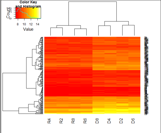
14. Plot the heatmap showing clustering of genes filtered in step 12. Save the heatmap image.

7.1.3.9 .

15. You are provided with an annotation file, anno.txt, of all the genes containing information of gene name, description and accession number. Retrieve the annotations for genes filtered in step 12 from anno.txt file. Hint: Search “%in%” in help and try to understand from the given example.

7.1.3.10 .

16. Group the genes as per their pathways. Arrange the values for each group according expression on D2. Write the arranged data in a file, Genes_arranged.txt.

7.2 Case study1: Solution

1. Import the file “path.txt” into R.

data=read.table("path.txt",header=T)

2. What is the data structure of imported file?

str(data)

3. How many rows and columns are there?

dim(data)

4. What are column names?

colnames(data)

5. Find out minimum, first quantile, median, third quantile, mean and maximum of expression values on each day. Store the result in a file.

summary(data)

6. Visualization of gene expression on 2,4,6,8 days of D and R plants using boxplot.

boxplot(data[,2:9]);

7. Visualization of pairwise correlation of gene expressions among R2, R4, R6 and R8.

pairs(data[,2:5],upper.panel=NULL)

8. Visualization of pairwise correlation of gene expressions among D2, D4, D6 and D8.

pairs(data[,6:9],upper.panel=NULL)

9. Calculate the pairwise correlation coefficient values among R2, R4, R6 and R8.

rcor=cor(data[,2:5])

10. Calculate the pairwise correlation coefficient values among D2, D4, D6 and D8.

dcor=cor(data[,6:9])

11. Draw a four panel plot depicting four scatterplots of R2 Vs D2, R4 Vs D4, R6 Vs D6 and R8 Vs D8.

par(mfrow=c(2,2))
plot(data$D2,data$R2,xlab="D2",ylab="R2",cex.lab=1.5);
plot(data$D4,data$R4,xlab="D4",ylab="R4",cex.lab=1.5);
plot(data$D6,data$R6,xlab="D6",ylab="R6",cex.lab=1.5);
plot(data$D8,data$R8,xlab="D8",ylab="R8",cex.lab=1.5);

12. Filter those genes that are up-regulated in D variety on all days i.e. (D2-R2)>0; (D4-R4)>0; (D6-R6)>0 and (D8-R8)>0. Write the differential expression values of these filtered genes in a file, up.txt.

library(dplyr)
# Filter those genes which are up/down regulated in Diseased condition.

temp=mutate(data,diff2=D2-R2,diff4=D4-R4,diff6=D6-R6,diff8=D8-R8,diff2up=diff2>0,diff4up=diff4>0,diff6up=diff6>0,diff8up=diff8>0,totup=diff2up+diff4up+diff6up+diff8up);

head(temp)
up3=filter(temp,totup>3);
write.table(up3,file="up.txt",sep="\t",eol="\n",quote=F,row.names=F)

13. Count the pathway wise gene count for the genes, which are filtered in step 12.

pathcount=table(up3$Path);

14. Plot the heatmap showing clustering of genes filtered in step 12. Save the heatmap image.

library("gplots");
h=heatmap.2(as.matrix(up3[,2:9]),trace="none")

15. You are provided with an annotation file, anno.txt, of all the genes containing information of gene name, description and accession number. Retrieve the annotations for genes filtered in step 12 from anno.txt file. Hint: Search “%in%” in help and try to understand from the given example.

annotation=read.table("anno.txt", sep="\t",header=T)
temp=annotation$Gene  %in% up3$Gene
info=annotation[temp,]

16 Group the genes as per their pathways. Arrange the values for each group according expression on D2. Write the arranged data in a file, Genes_arranged.txt.

gengrp=group_by(up3, Path)
arr=arrange(gengrp,D2)
write.table(arr,"Genes_arranged.txt", sep="\t", quote = F)

7.3 Tasks

7.3.1 Vector creation

1. Create a vector x13 with values 2, 3, 4, 5, 6
2. Create a vector x14 with values 2.0, 2.1, 2.2, 2.3, 2.4, .., 4
3. Create a vector x15 with 10 random values between 4 and 6
4. Create a vector x16 with repeated values 3, 4, 5, 3, 4, 5, 3, 4, 5
5. Create x17 with repeated values 7,7,7,8,8,8,9,9,9
6. Create a vector x18 with 10 random values between 20 and 30
7. Create a vector x19 with 10 normally distributed random values
8. Create a vector x20 with values of vectors x13 and x16 followed by 3, 5,10

7.3.2 Fetching vector elements

9. Create a vector x21 with values 33,55,66,88,99. Fetch its 3rd, 5th and 2nd values
10. Fetch values of x21 from 1 to 4
11. Fetch values of x21 vector excluding 2nd and 3rd elements 12 Fetch last element of x21 using length()

7.3.3 Vector manipulation

13. Create a vector x23 with values 5, 7, 6, 8, 1, 4. Delete 1st and last element. Reset the value of second element to 12. Add value 0 at the beginning of a vector x

7.3.4 Vector arithmetic

14. Write the arithmetic expression to calculate variance of a vector. Cross check your result using var() function. Formula: Variance= sum((x-mean(x))^2) /n-1 where n is total number of elements.
15. Given x, y, z coordinates of two atoms. Atom1 (1.2, 2.3, 3.4) and Atom2 (4.5, 5.6, 6.7). Find distance between 2 atoms. Formula: sqrt((x2-x1)^2+(y2-y1)2+(z2-z1)^2)
16. Find out the numbers between 1 to 100, which are divisible by 2 or 3.

7.3.5 Matrix

17. Create a matrix from a vector consisting of numbers from 1 to 12 with 3 columns
18. Fetch 2nd row. Fetch 3rd column
19. Fetch the value 6
20. Fetch the value 8 and 12
21. Fetch the value 7, 8, 11 and 12

7.3.6 Data Frame

22. Create a data frame of gene expression data such that

First column,“Genes”, is a character vector of 6 gene names (G1, G2, …, G6).

Second column, “C1” is a numeric vector of 6 random values from 3 to 5.

Hint: Generate random numbers using function sample(). Use R help to see the syntax of sample.

Third column, “C2” is a numeric vector of 6 random values from 3 to 5.

Fourth column, “T1” is a numeric vector of 6 random values from 5 to 7.

Fifth column, “T2” is a numeric vector of 6 random values from 5 to 7.

Sixth column, “Pathway” is a character vector of which first 3 represent one pathway “P1” and other 3 represent pathway “P2”.

23. Fetch values of column T2
24. Fetch values of gene G2
25. Fetch value of gene G3 from C2
26. Delete column C2
27. Insert column C3, which should be numeric vector of 6 random values from 3 to 5.
28. Find mean of column C1

7.3.7 Tasks on Iris data set

1. Open iris data set file using read.table() and store in a variable names “iris_data”
2. Check the structure of “iris_data”. Note the column names. How many categories are there in column named as “Species”. Note the names of species.
3. How many rows and columns are there?
4. How many observations (rows) are there for each species?

1. Number of rows with Species as setosa
2. Number of rows with Species as virginica
3. Number of rows with Species as versicolor

5. Find the mean of all sepal lengths.
6. Find the mean of sepal lengths in Species setosa.
7. What is the overall correlation between Sepal length and Petal length?
8. What is the correlation between Sepal width and Petal width of Species virginica?
9. Find the difference between sepal lengths of species setosa and versicolor. What is the mean difference between them?
10. Carry out the t-test between sepal lengths of species setosa and versicolor. Is it statistically significant?

7.3.8 Visualization

You are provided with an excel file “iris.xls”. The file contains IRIS data, 150 flowers, Categorized into 3 plants (SP:Setosa/Versicolor/Virginica) and two colors (Col:Red/Blue).

The data consists of SL (Sepal length), SW (Sepal width), PL (Petal length) and PW (Petal width) in cm.

Task: Load the data in R using appropriate function and extract useful information by data visualization.

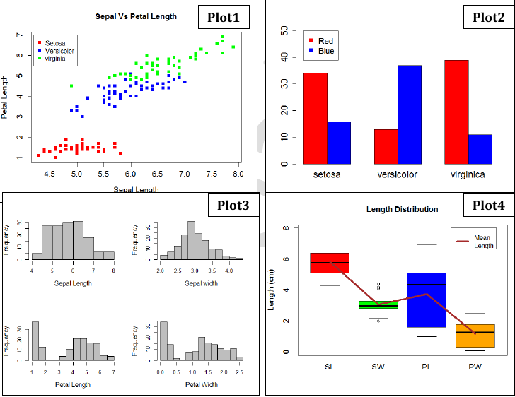
• Plot1: Scatter plot of Sepal length vs Petal length of all 150 flowers, color according to species/plants.
• Plot2: Barplot showing distribution of Sepal lengths among 6 classes of flowers (3 plants and 2 colors).
• Plot3: Multi panel plot showing the histogram of SL, PL, SW, PW of all 150 flowers.
• Plot4: Box plot showing SL, SW, PL, PW distribution along with a line joining their mean lengths.

• Plot5: Probability density plot of Sepal lengths among three different categories of plants.
• Plot6: 3D plot showing distinct clustering of flowers in terms of SL, SW and PL. Different colors for different plants.

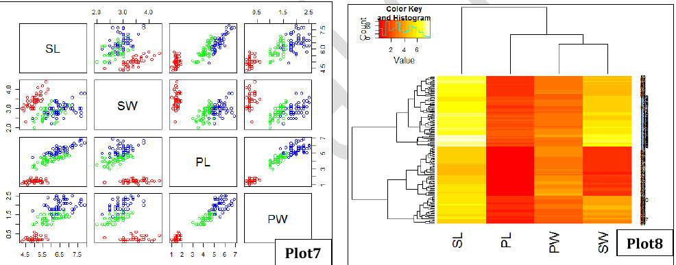
• Plot7: Scatter plot matrix showing a global view of the distribution of SL, SW, PL and PW across 3 plants.
• Plot8: Heatmap showing clustering of flowers in terms of their SL, SW, PL and PW properties.

• Plot9: Pie chart showing the number of flowers in 6 categories (3 plants and 2 colors)
• Plot10: Dot chart showing clear distribution of SL among 3 plants.

7.4 Solutions

7.4.1 Vector creation

1. Create a vector x13 with values 2, 3, 4, 5, 6

x13=c(2,3,4,5,6)

2. Create a vector x14 with values 2.0, 2.1, 2.2, 2.3, 2.4, .., 4

x14=seq(from=2,to=4, by=0.1)

3. Create a vector x15 with 10 random values between 4 and 6

x15=sample(4:6,10, replace=T)

4. Create a vector x16 with repeated values 3, 4, 5, 3, 4, 5, 3, 4, 5

x16=rep(c(3,4,5),times=3)

5. create x17 with repeated values 7,7,7,8,8,8,9,9,9

x17=rep(c(7,8,9),each=3)

6. Create a vector x18 with 10 random values between 20 and 30

x18=sample(20:30,10)

7. Create a vector x19 with 10 normally distributed random values

x19=rnorm(10)

8. Create a vector x20 with values of vectors x13 and x16 followed by 3, 5,10

x20=c(x13,x16,3,5,10)

7.4.2 Fetching vector elements

9. Create a vector x21 with values 33,55,66,88,99 and fetch its 3rd, 5th and 2nd values

x21=c(33,55,66,88,99)

x21[c(3,5,2)]

10. Fetch its values from 1 to 4

x21[1:4]

11. Fetch values of x21 vector excluding 2nd and 3rd elements

x22=x21[-c(2,3)]

x22

12 Fetch last element of x21 using length()

x21[length(x21)]

7.4.3 Vector manipulation

13. Create a vector x23 with values 5, 7, 6, 8, 1, 4.

x23=c(5,7,6,8,1,4)

Delete 1st and last elements.

x23=x23[-c(1,length(x23))]

Reset the value of second element to 12.

x23[2]=12

Add value 0 at the beginning of a vector x23

x23=c(0,x23)

7.4.4 Vector arithmetic

14. Calculate Variance

Write the arithmetic expression to calculate variance of a vector. Cross check your result using var() function.

Formula: Variance= sum((x-mean(x))^2) /n-1 where n is total number of elements.

x=c(5,7,6,8,1,4)

xvar=sum((x-mean(x))^2)/(length(x)-1)

xvar

var(x)

15. Distance between atoms

Given x, y, z coordinates of two atoms. Atom1 (1.2, 2.3, 3.4) and Atom2 (4.5, 5.6, 6.7). Find distance between 2 atoms. Formula: sqrt((x2-x1)2+(y2-y1)2+(z2-z1)2)

atom1=c(1.2,2.3,3.4)

atom2=c(4.5,5.6,6.7)

dist=sum((atom1-atom2)^2)

dist

16. Find out the numbers between 1 to 100, which are divisible by 2 or 3.

x=1:100

x[which(x%%2==0 & x%%3==0)]

7.4.5 Matrix

17 Create matrix

Create a matrix from a vector cosisting of numbers from 1 to 12 with 3 columns

mt=matrix(1:12,ncol=3)

18. Fetch 2nd row. Fetch 3rd column

mt[2,]

mt[,3]

19. Fetch the value 6

mt[2,2]

20. Fetch the value 8 and 12

mt[4,c(2,3)]

21. Fetch the value 7, 8, 11 and 12

mt[c(3,4),c(2,3)]

7.4.6 Data Frame

22. Create a data frame of gene expression data such that

First column,“Genes”, is a character vector of 6 gene names (G1, G2, …, G6).

Second column, “C1” is a numeric vector of 6 random values from 3 to 5.

Hint: Generate random numbers using function sample(). Use R help to see the syntax of sample.

Third column, “C2” is a numeric vector of 6 random values from 3 to 5.

Fourth column, “T1” is a numeric vector of 6 random values from 5 to 7.

Fifth column, “T2” is a numeric vector of 6 random values from 5 to 7.

Sixth column, “Pathway” is a character vector of which first 3 represent one pathway “P1” and other 3 represent pathway “P2”.

genes=paste(“G”,1:6,sep="")

C1=sample(3:5,6, replace=T)

C2=sample(3:5,6, replace=T)

T1=sample(5:7,6, replace=T)

T2=sample(5:7,6, replace=T)

pathway=rep(c(“P1”,“P2”),each=3)

exp=data.frame(“Genes”=genes,“C1”=C1,“C2”=C2,“T1”=T1,“T2”=T2,“Pathway”=pathway)

23. Fetch values of column D2

exp$T2

24. Fetch values of gene G2

exp[2,]

25. Fetch value of gene G3 from C2

exp[3,3]

26. Delete column C2

exp$C2=NULL

27. Insert column C3, which should be numeric vector of 6 random values from 3 to 5.

exp$C3=sample(3:5,6, replace=T)

28. Find mean of column C1

mean(exp$C1)

7.4.7 Tasks on iris data set

1. Open iris data set file using read.table() and store in a variable name “iris_data”

iris_data=read.table(“iris.txt”,header=T)

2. Check the structure of “iris_data”. Note the column names. How many categories are there in column named as “Species”. Note the names of species.

str(iris_data)

levels(iris_data$Species)

3. How many rows and columns are there?

dim(iris_data)

4. How many observations (rows) are there for each species?

a. Number of rows with Species as setosa

b. Number of rows with Species as virginica

c. Number of rows with Species as versicolor

table(iris_data$Species)

5. Find the mean of all sepal lengths.

mean(iris_data$Sepal.Length)

6. Find the mean of sepal lengths in Species setosa.

library(dplyr)

setosa=filter(iris_data, Species==“setosa”)

mean(setosa$Sepal.Length)

7. What is the overall correlation between Sepal length and Petal length?

cor(iris_data$Sepal.Length, iris_data$Petal.Length)

8. What is the correlation between Sepal width and Petal width of Species virginica?

virginica=filter(iris_data, Species==“virginica”)

cor(virginica$Sepal.Width, virginica$Petal.Width)

9. Find the difference between sepal lengths of species setosa and versicolor. What is the mean difference between them?

versicolor=filter(iris_data, Species==“versicolor”)

sldiff= setosa$Sepal.Length - versicolor$Sepal.Length

mean(sldiff)

10. Carry out the t-test between sepal lengths of species setosa and versicolor. Is it statistically significant?

Assumptions: Sepal lengths of two species are normally distributed Their variances may not be equal Observations are not paired Two sided t-test, we are just interested to know if sepal lenghts between species are significantly different or not.

t.test(setosa$Sepal.Length, versicolor$Sepal.Length)

Based on p-value we reject null hypothesis at 95 % confidence interval Hence sepal lengths of species setosa and versicolor are significantly different

Note: Please see the help for t.test to find out various options for t-test

7.4.8 Visualization

Plot1: Scatter plot of Sepal length vs Petal length of all 150 flowers, color according to species/plants.

library(gdata)
irisd=read.xls("iris.xls");

plot(irisd$SL,irisd$PL,col=rep(c("red","blue","green"),each=50),pch=15,xlab="Sepal Length",ylab="Petal Length",cex.lab=1.2,main="Sepal Vs Petal Length",cex.axis=1.2)
legend(4.2,7,c("Setosa","Versicolor","virginia"),col=c("red","blue","green"),pch=15)

Plot2: Barplot showing distribution of Sepal lengths among 6 classes of flowers (3 plants and 2 colors).

barplot(t(table(irisd$SP,irisd$Col)),beside=T,col=c("red","blue"),ylim=c(0,50),cex.axis=1.5,cex.name=1.5)
legend(1,50,c("Red","Blue"),pch=15,col=c("red","blue"))

Plot3: Multi panel plot showing the histogram of SL, PL, SW, PW of all 150 flowers.

par(mfrow=c(2,2))
hist(irisd[,1],xlab="Sepal Length",ylab="Frequency",main="",cex.lab=1.2,col="gray")
hist(irisd[,2],xlab="Sepal width",ylab="Frequency",main="",cex.lab=1.2,col="gray")
hist(irisd[,3],xlab="Petal Length",ylab="Frequency",main="",cex.lab=1.2,col="gray")
hist(irisd[,4],xlab="Petal Width",ylab="Frequency",main="",cex.lab=1.2,col="gray")
par(mfrow=c(1,1))

Plot4: Box plot showing SL, SW, PL, PW distribution along with a line joining their mean lengths.

boxplot(irisd[,1:4],col=c("red","green","blue","orange"),main="Length Distribution",cex.axis=1.2,ylab="Length (cm)",cex.lab=1.2)
l=summarise(irisd,mean(SL),mean(SW),mean(PL),mean(PW))
lines(c(1,2,3,4),l,lwd=4,col="brown")
legend(3.5,8,c("Mean\nLength"),lty=1,lwd=4,col="brown")

Plot5: Probability density plot of Sepal lengths among three different categories of plants.

# First filter
library(dplyr)
set_SL=filter(irisd,SP=="setosa") %>% select(SL)
versi_SL=filter(irisd,SP=="versicolor") %>% select(SL)
virgi_SL=filter(irisd,SP=="virginica") %>% select(SL)

# Convert them to vector
set_SL=set_SL$SL
versi_SL=versi_SL$SL;
virgi_SL=virgi_SL$SL;


# use density to plot
plot(density(set_SL),xlim=c(4,10),lwd=2,xlab="Length (cm)",main="Prob. Density of Sepal Length across different flowers")
lines(density(versi_SL),col="red",lwd=2)
lines(density(virgi_SL),col="green",lwd=2)
legend(8,1.2,lwd=2,c("Setosa","Versicolor","Virginica"),col=c("black","red","green"))

Plot6: 3D plot showing distinct clustering of flowers in terms of SL, SW and PL. Different colors for different plants.

library(rgl)
plot3d(irisd[,1:3],col=rep(c("red","green","blue"),each=50))

Plot7: Scatter plot matrix showing a global view of the distribution of SL, SW, PL and PW across 3 plants.

pairs(irisd[,1:4],col=rep(c("red","green","blue"),each=50))

Plot8: Heatmap showing clustering of flowers in terms of their SL, SW, PL and PW properties.

m=as.matrix(irisd[,1:4]);
library("gplots")
heatmap.2(m, trace="none")

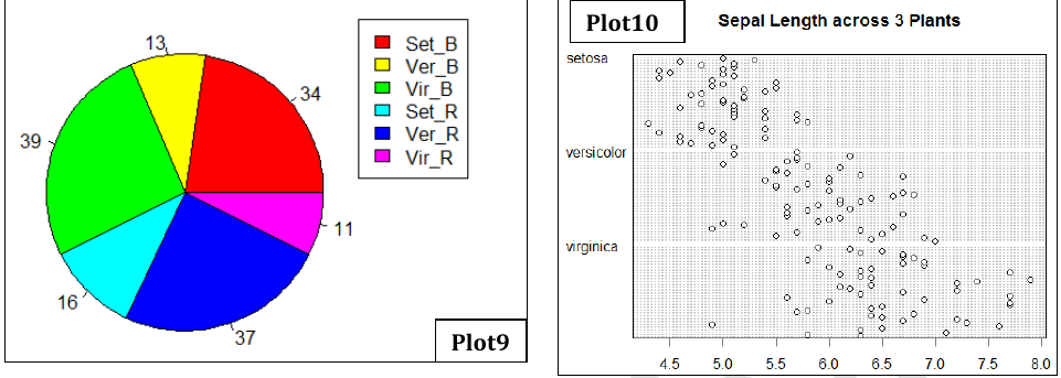
Plot9: Pie chart showing the number of flowers in 6 categories (3 plants and 2 colors)

#Subset species by colors
library(dplyr)

Set_B=filter(irisd, SP=="setosa" & Col=="Blue" )
Set_R=filter(irisd, SP=="setosa" & Col=="Red" )
Ver_B=filter(irisd, SP=="versicolor" & Col=="Blue" )
Ver_R=filter(irisd, SP=="versicolor" & Col=="Red" )
Vir_B=filter(irisd, SP=="virginica" & Col=="Blue" )
Vir_R=filter(irisd, SP=="virginica" & Col=="Red" )

#Create vector of counts in each subset
irisp=c(nrow(Set_B),nrow(Set_R),nrow(Ver_B),nrow(Ver_R),nrow(Vir_B),nrow(Vir_R))

pie(irisp, labels=irisp, col=c("Red", "Cyan", "yellow", "Blue", "Green", "Magenta"))
legend(0.9,1,c("Set_B","Ver_B","Vir_B","Set_R","Ver_R","Vir_R"),pch=15, col=c("Red","Yellow","Green", "Cyan","Blue","Magenta"))

Plot10: Dot chart showing clear distribution of SL among 3 plants.

dotchart(irisd$SL,group=irisd$SP, main="Sepal Length across 3 Plants")