Descriptive_statistics

Measure of Centrality (Mean, Median), summary and quantile function

data=c(11,2,35,46,55);
print(data);

## [1] 11  2 35 46 55

mean(data); # Estimate mean

## [1] 29.8

median(data); # Estimate median

## [1] 35

summary(data); # Summarise the data

##    Min. 1st Qu.  Median    Mean 3rd Qu.    Max. 
##     2.0    11.0    35.0    29.8    46.0    55.0

quantile(data); # Estimate quartiles

##   0%  25%  50%  75% 100% 
##    2   11   35   46   55

quantile(x = data, probs = 0.25); # First quantile

## 25% 
##  11

quantile(x = data, probs = 0.5); # Second quantile or Median

## 50% 
##  35

quantile(x = data, probs = 0.75); # Third quantile

## 75% 
##  46

# Percentile
quantile(x = data, probs = c(0.30, 0.45, 0.65)); # 30th, 45th and 65th percentile

##  30%  45%  65% 
## 15.8 30.2 41.6

Measure of Spread (Variance, Standard deviation, Range, IQR)

var(data); # Variance

## [1] 512.7

sd(data); # Standard deviation

## [1] 22.64288

range(data); # range, returns min and max

## [1]  2 55

max(data) - min(data); # Range

## [1] 53

IQR(data); # Inter quartile range

## [1] 35

# Estimate IQR by yourself, IQR= quantile3-quantil1 i.e. Q3-Q1
# Compare the result with the result of IQR function
q1 = quantile(x = data, probs = 0.25); # First quantile
q3 = quantile(x = data, probs = 0.75); # Third quantile
print(q3-q1);

## 75% 
##  35

Missing values if present in the data, use na.rm parameter

# Before adding NA, data:
print(data);

## [1] 11  2 35 46 55

# Add one missing value at the end
data=c(data,NA);
# After adding NA, data:
print(data);

## [1] 11  2 35 46 55 NA

mean(data); # without na.rm parameter, if Na is present result will be NA

## [1] NA

mean(data, na.rm = TRUE); # with na.rm parameter, if NA is present, then they are excluded

## [1] 29.8

# u have to use na.rm in median, var, sd, IQR, range, quantile function
summary(data); # no need to give na.rm, NA are treated separately

##    Min. 1st Qu.  Median    Mean 3rd Qu.    Max.    NA's 
##     2.0    11.0    35.0    29.8    46.0    55.0       1

Look at the distribution of iris dataset by ploting

# Consider iris dataset
head(iris); 

##   Sepal.Length Sepal.Width Petal.Length Petal.Width Species
## 1          5.1         3.5          1.4         0.2  setosa
## 2          4.9         3.0          1.4         0.2  setosa
## 3          4.7         3.2          1.3         0.2  setosa
## 4          4.6         3.1          1.5         0.2  setosa
## 5          5.0         3.6          1.4         0.2  setosa
## 6          5.4         3.9          1.7         0.4  setosa

# Check sepal length distribution
# Since sepal length is numerical data, we can use hist() and density() to see the distribution

# Histogram
hist(iris$Sepal.Length, xlab="Sepal Length", main="Histogram of Sepal Length");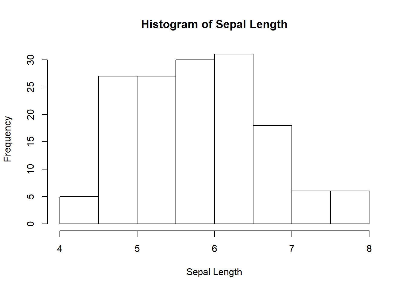

# Density plot
# You can see its a unimodal distribution
plot(density(iris$Sepal.Length), xlab="Sepal Length", main="Density of Sepal Length")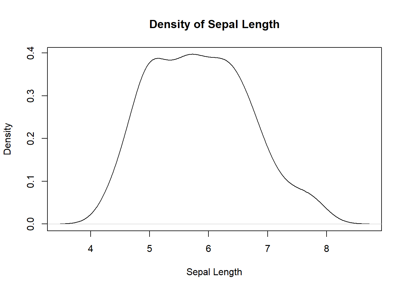

# Box plot
boxplot(iris$Sepal.Length, main="Boxplot of Sepal Length")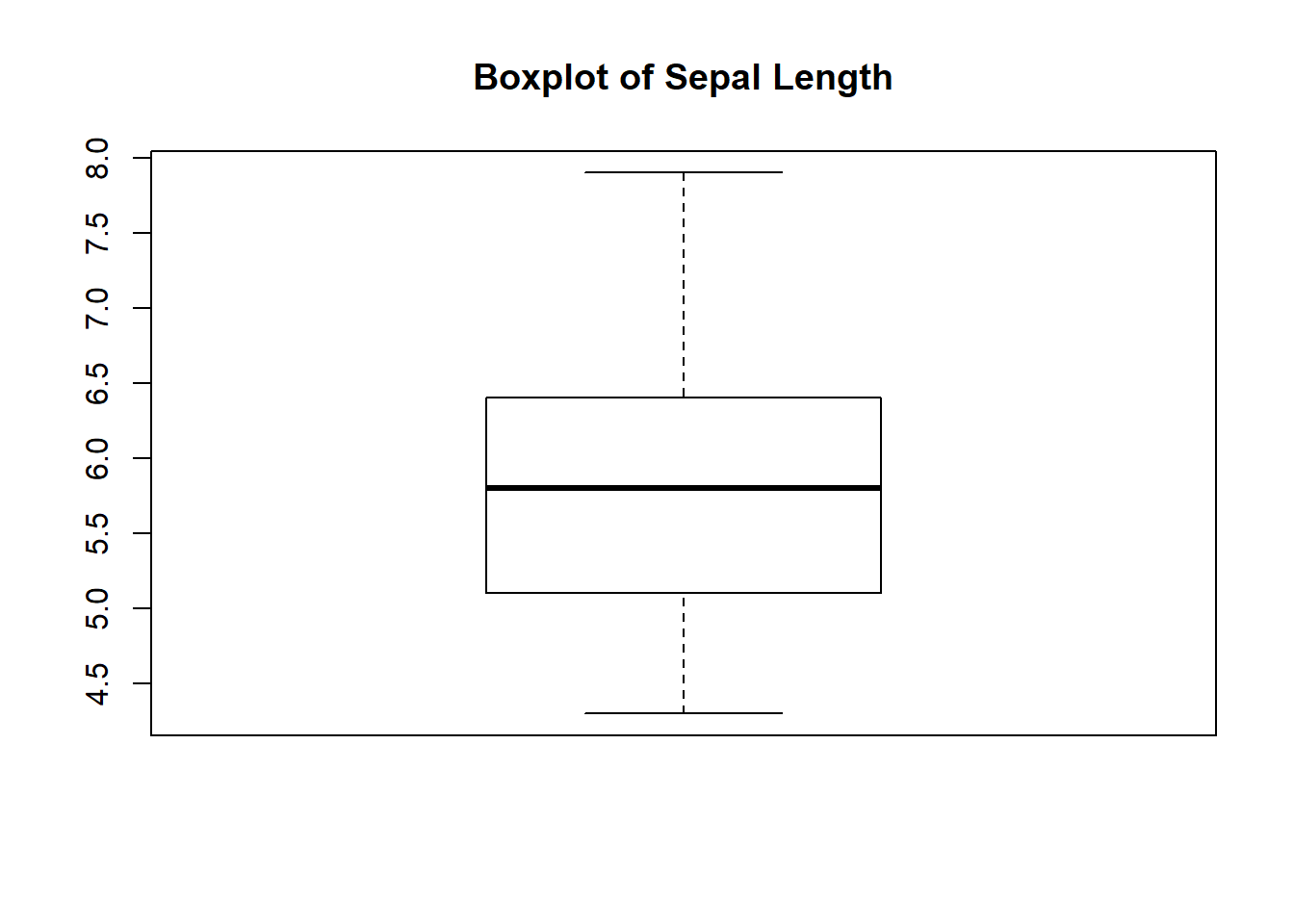

# Histogram of four features (Sepal.Length Sepal.Width Petal.Length Petal.Width) of iris dataset
par(mfrow=c(2,2));
hist(iris$Sepal.Length, xlab="Sepal Length", main="Histogram of Sepal Length")
hist(iris$Sepal.Width, xlab="Sepal Width", main="Histogram of Sepal Width")
hist(iris$Petal.Length, xlab="Petal Length", main="Histogram of Petal Length")
hist(iris$Petal.Width, xlab="Petal Width", main="Histogram of Petal Width")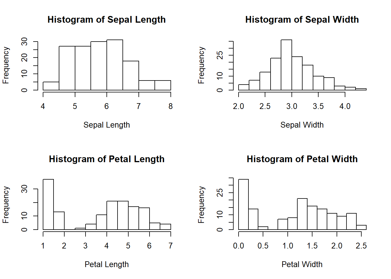

# Density plot of four features (Sepal.Length Sepal.Width Petal.Length Petal.Width) of iris dataset
par(mfrow=c(2,2));
plot(density(iris$Sepal.Length), xlab="Sepal Length", main="Density plot of Sepal Length")
plot(density(iris$Sepal.Width), xlab="Sepal Width", main="Density plot of Sepal Width")
plot(density(iris$Petal.Length), xlab="Petal Length", main="Density plot of Petal Length")
plot(density(iris$Petal.Width), xlab="Petal Width", main="Density plot of Petal Width")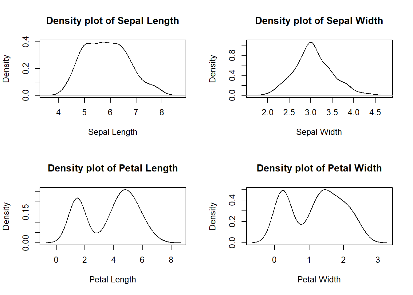

# Box plot of four features (Sepal.Length Sepal.Width Petal.Length Petal.Width) of iris dataset
par(mfrow=c(1,1));
boxplot(iris[,1:4])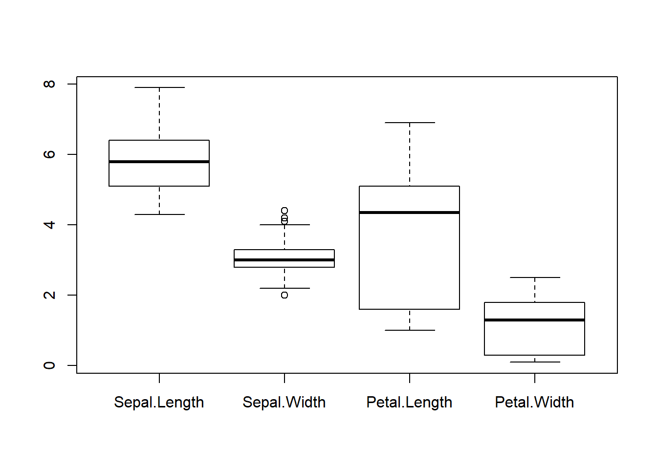

# Density plot of four features (Sepal.Length Sepal.Width Petal.Length Petal.Width) of iris dataset. Mean is marked in red line while median in blue.
par(mfrow=c(2,2));
plot(density(iris$Sepal.Length), xlab="Sepal Length", main="Density plot of Sepal Length")
meanval= mean(iris$Sepal.Length)
medianval=median(iris$Sepal.Length);
lines(c(meanval, meanval),c(0,1), lwd=2, col="red"); # mean line
lines(c(medianval, medianval),c(0,1), lwd=2, col="blue"); # mean line

plot(density(iris$Sepal.Width), xlab="Sepal Width", main="Density plot of Sepal Width")
meanval= mean(iris$Sepal.Width)
medianval=median(iris$Sepal.Width);
lines(c(meanval, meanval),c(0,1), lwd=2, col="red"); # mean line
lines(c(medianval, medianval),c(0,1), lwd=2, col="blue"); # mean line

plot(density(iris$Petal.Length), xlab="Petal Length", main="Density plot of Petal Length")
meanval= mean(iris$Petal.Length)
medianval=median(iris$Petal.Length);
lines(c(meanval, meanval),c(0,1), lwd=2, col="red"); # mean line
lines(c(medianval, medianval),c(0,1), lwd=2, col="blue"); # mean line

plot(density(iris$Petal.Width), xlab="Petal Width", main="Density plot of Petal Width")
meanval= mean(iris$Petal.Width)
medianval=median(iris$Petal.Width);
lines(c(meanval, meanval),c(0,1), lwd=2, col="red"); # mean line
lines(c(medianval, medianval),c(0,1), lwd=2, col="blue"); # mean line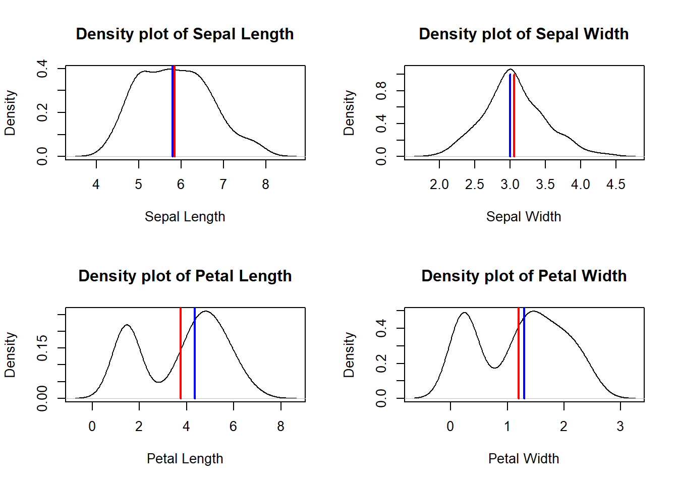

Estimate Skewness and Kurtosis

Load the moments library

library(moments);  

Calculate skewness. Skewness is a measure of symmetry.

Negative skewness: mean of the data < median and the data distribution is left-skewed.

Positive skewness: mean of the data > median and the data distribution is right-skewed.

skewness(iris$Sepal.Length); # distribution is skewed towards the right. 

## [1] 0.3117531

skewness(iris$Sepal.Width); # distribution is skewed towards the right. 

## [1] 0.3157671

skewness(iris$Petal.Length); # distribution is skewed towards the left. 

## [1] -0.2721277

skewness(iris$Petal.Width); # distribution is skewed towards the left. 

## [1] -0.1019342

Estimate kurtosis. kurtosis describes the tail shape of the data distribution.

The normal distribution has zero kurtosis and thus the standard tail shape. It is said to be mesokurtic.

Negative kurtosis would indicate a thin-tailed data distribution, and is said to be platykurtic.

Positive kurtosis would indicate a fat-tailed distribution, and is said to be leptokurtic.

kurtosis(iris$Sepal.Length);

## [1] 2.426432

kurtosis(iris$Sepal.Width);

## [1] 3.180976

kurtosis(iris$Petal.Length);

## [1] 1.604464

kurtosis(iris$Petal.Width);

## [1] 1.663933